RAMSES Code
This is a documentation and tutorial guideline for compilation of the RAMSES code, particularly on Sedov-Taylor Astronomical Problem and the application of High Performance Computing (HPC). This is a simple guide to under the Sedov-Taylor theory and generating a GIF-like animation for 1D, 2D and 3D input files, and it lays out the exact procedure I followed, because initially it might confuse anyone. I have performed only the Sedov input code, just to check how RAMSES works and what we can extract from this tool. I am interested in combining astronomical calculations with HPC in the future. To show off this interest and curiosity of mine, I tried running a job on the “Comet” HPC cluster provided by Newcastle University. As the Sedov 3D data is a very large, which will take a long period to run on local machine. This is one best reason to combine HPC in this workflow, as I was able to get a satisfactory output via accessing the cluster.
Up to this point, I have compiled 1D on my local machine T430, while 2D and 3D on 'Comet' HPC cluster. HPC does a great job in processing the data in short period. The major aim of documenting this is to see the animation at the end of compiling the RAMSES code. I personally feel that without seeing an animation, it was a little boring for me. Hence, here is a simple guide on 'how I got an animation of 2D and 3D Sedov code for different timelines' and 'how to submit a slurm job on cluster'. I have also attached the actual task pictures with step-by-step procedures for better understanding and easier guidance.
1 Introduction:
1.1 Basics of RAMSES Code:
Ramses Code is an open-source project code, written in Fortran programming languages. Its mainly used to study some various properties of the evolving universe by modeling phenomena like some explosion, gravitation, magnetization, any radiation caused and many more other astrophysical processes. Ramses models these astronomical simulation and complex calculation to help researchers better understand these systems. It is widely used in cosmology and galaxy formation studies. The code is parallelized using MPI, which makes it suitable for high-performance computing (HPC) clusters and large-scale simulations. Ramses uses Adaptive Mesh Refinement (AMP) techniques, but What is (AMR)? Its a simulations techniques that focuses a specified area with more computing power and refined scale to capture more detailing a particular ares. This makes simulations more efficient and accurate without wasting CPU and memory by using coarser grids in less important regions. This overview provides sufficient background to begin working with RAMSES, but if you want to learn in more detail, you can visit the official documentation page official here
1.2 What is Sedov-Taylor-von Neumann?:
The “Sedov-Taylor-von Neumann” is a mathematical and physical model used to describe how a strong explosion spreads out in a gas or fluid. As its modeling to understand a explosion is theorized as blast wave. When an explosion occurs it releases a huge amounts of a shock wave outward. and This shocks wave are actually studied using mathematical formula and using physics theory to understand universe thats it. This model explains how the shock wave is behaving with time, like changes in position, density, velocity, pressure, temperature etc. This model is fundamental in astrophysics and fluid dynamics because it helps us to understand explosions caused by supernovae, nuclear blasts, or any sudden energy release in universe. This is named after three scientists, Leonid Sedov, G. I. Taylor and John von Neumann, and submitted their research on similar problem. In the Sedov–Taylor–von Neumann model, we consider a very strong explosion that releases a large amount of energy (E) in a very small region over a small period of time. This sudden release of energy produces a spherical shock wave that moves outward from the center of the explosion. When the shock wave has traveled far enough distance, the exact size and duration of the original explosion no longer affect its behavior. Instead, the evolution of the shock depends only on the total released energy (E) and the density of the surrounding gas (ρ). For simplicity, let us assume that the explosion occurs at a single point of radius=0 at time (t=0), and that the surrounding medium has a uniform density. Because the shock wave is very strong, the pressure ahead of the shock can be neglected, but the surrounding density cannot be ignored, since the shock sweeps up this material as it expands. The gas is treated as an ideal gas with a specific heat ratio (γ), which allows the physical properties behind the shock to be calculated using conservation laws. Shock Radius: This explains “how far the explosion spreads. The shock radius evolves as Using dimensional analysis, the only meaningful combination of the variables, radius (r), time (t), and energy (E) and density in front of the shock (ρ),
R(t) = β (E t2 / ρ0)1/5
This equations tells us that the shock radius increases as time passes, meaning the explosion continues to expand outward. It also shows that a larger explosion energy results in a larger shock radius at any given time, since more energy pushes the shock farther into the surrounding medium. On the other hand, if the surrounding gas has a higher density, the expansion becomes slower because the shock wave has to move more mass as it propagates outward. you can have a visit at this page here.
2 Requirements:
Before starting, I highly recommend using a Linux distribution, as its way much easier to figure out the problems. As for compiling RAMSES code, we will need some packages installed on our system such as:
git: To install and manage git code. I have git (2.52.0-2) installed in my system. If you're using an Arch-based system, you can install 'git' via below command:
This command will let you search all the git package,sudo pacman -S gitsudo pacman -Ss gitgfortran: To compile and run Ramses Code, we will typically need a Fortran compiler installed on our system. I have 'gfortran' (15.2.1) preinstalled in my distro. This Fortran will help us to get a executable file for ramses 1D, 2D, and 3D. However, if you can search using this command flag '-Ss'. I get this following output, which means, I have it preinstalled in my system.
[golu@T430 ~]$ sudo pacman -Ss gfortran
core/gcc-libs 15.2.1+r447+g6a64f6c3ebb8-1 [installed: 15.2.1+r301+gf24307422d1d-1]
Runtime libraries shipped by GCC
core/lib32-gcc-libs 15.2.1+r447+g6a64f6c3ebb8-1 [installed: 15.2.1+r301+gf24307422d1d-1]
32-bit runtime libraries shipped by GCC
Note: Basicallly gfortran and python should be your system installation. One reason why Linux is great, it usually comes with important tools, packages and libraries already set up for you.
python: To visualizTo visualize the RAMSES output in image or GIF format, you will need 'python' (version 3.11.0 or higher) along with some required libraries such as Osyris and Pynbody. First you need to make a working directory using this below command, mine is simply 'ramses', then use cd command to change directory the RAMSES output in image or GIF format, you will need 'python' (version 3.11.0 or higher) along with some required libraries such as Osyris and Pynbody. First you need to make a working directory using this below command, mine is simply 'ramses', then use cd command to change directory.
mkdir <directory_name>
cd <directory_name>
Python Virtual Environment: Once you are inside this directory, you can check your path using command 'pwd'. Now its important to note that Python libraries cant be installed without having a python virtual environment and neither it works without it. You can create a virtual environment using this command where 'mynewvenv' will create you a directory.
This is where you installed the python libraries. Now you need to activate this virtual environment using below command,python -m venv mynewvenv
One activated, you will see a prompt near the name, like below,source mynewvenv/bin/activate
Now you are ready to install python package, using this command and once done,(mynewvenv)[golu@T430 ramses] $
You will see this output as shown in the image, which tell you what other packages has been installed.pip install osyris pynbodyRamses Code: You need to git clone in the working directory, this will download latest GitHub repository here.
You can check listing using 'ls' command, here the blue shows me directories while green shows me a text file.(mynewvenv)[golu@T430 ~]$ git clone https://github.com/ramses-organisation/ramses Cloning into 'ramses'... remote: Enumerating objects: 26381, done. remote: Counting objects: 100% (188/188), done. remote: Compressing objects: 100% (104/104), done. remote: Total 26381 (delta 122), reused 84 (delta 84), pack-reused 26193 (from 2) Receiving objects: 100% (26381/26381), 98.70 MiB | 846.00 KiB/s, done. Resolving deltas: 100% (17894/17894), done.
You can also upgrade the pip version.Successfully installed certifi-2026.2.25 charset_normalizer-3.4.4 contourpy-1.3.3 cycler-0.12.1 flexcache-0.3 flexparser-0.4 fonttools-4.61.1 h5py-3.15.1 idna-3.11 kiwisolver-1.4.9 llvmlite-0.46.0 matplotlib-3.10.8 numba-0.64.0 numpy-2.4.2 osfclient-0.0.5 osyris-3.2.0 packaging-26.0 pillow-12.1.1 pint-0.25.2 platformdirs-4.9.2 pynbody-2.4.1 pyparsing-3.3.2 python-dateutil-2.9.0.post0 requests-2.32.5 scipy-1.17.1 six-1.17.0 tqdm-4.67.3 typing-extensions-4.15.0 urllib3-2.6.3 [notice] A new release of pip is available: 25.3 -> 26.0.1 [notice] To update, run: pip install --upgrade pip
3 Preparation of RAMSES code:
Here, We need a executable file for all dimensions, ramses1d, ramses2d and ramses3d, each has different Ramses code. We will first need to prepare the ’Makefile’ in this path (ramses/bin), you need to type
cd bininside directory where you just cloned the Ramses code.( mynewvenv ) [ golu@T430 ramses ] $ cd bin / ( mynewvenv ) [ golu@T430 bin ] $ ls clusters . mk Makefile ( mynewvenv ) [ golu@T430 bin ] $Here, we will edit “Makefile” using vim text editor. Basically we will just add two parameters, F90, which are now empty and other FFLAGS in the ’Makefile’ and we set this below value to F90 to gfortran as the Fortran compiler, and FFLAGS to add optimization and compatibility options so RAMSES compiles correctly and runs efficiently. You can download this Makefile from scripts directory also.
F90 = gfortran - O3 - frecord - marker =4 - fbacktrace - ffree - line - length - none
FFLAGS = -x f95 - cpp - input - DWITHOUTMPI $ ( DEFINES )
Also we need to check the following parameters for “Compilation time parameters”.
Compilation time parameters
NVECTOR = 64
NDIM = 1
NPRE = 8
NVAR = 8
SOLVER = hydro
PATCH =
EXEC = ramses
3.1 Executable File:
- Once all checked, save the file and we will compile the “Makelfile”. First we will clean the folder using this command ’make clean’ command and then re build the program.
Once finished, you will see something like this below( mynewvenv ) [ golu@T430 bin ] $ make clean rm -f *. o *. mod *. i
Here ’make clean’ command removes old compiled files, and ’make’ command compiles the program again to create fresh executable. Now you can check “ramses1d” filename.Ito-wrapper: warning: using serial compilation of 18 LTRANS jobs Ito-wrapper: note: see the ‘—flto’ option documentation for more information rm write_makefile.f9@ rm write_patch.f9[golu@T430 bin]$ ls adaptive_loop.o const.mod hydro_commons.o mpi_mod.mod poisson_parameters.o star_formation.o add_list.o cooling_fine.o hydro_flag.o mpi_mod.o ramses1d stellar_particle.o amr_commons.mod cooling_module_ism.o hydro_parameters.mod multigrid_fine_coarse.o synchro_fine.o amr_commons.o cooling_module.mod hydro_parameters.o multigrid_fine_commons.o synchro_hydro_fine.o amr_constants.mod cooling_module.o init_amr.o multigrid_fine_fine.o ramses.o timer_m.mod amr_constants.o courant_fine.o init_flow_fine.o nbors_utils.o random.mod timer.o amr_parameters.mod dump_utils.mod init_hydro.o newdt_fine.o random.o title.o amr_parameters.o dump_utils.o init_part.o output_amr.o read_hydro_params.o tracer_utils.mod amr_step.o end.o init_poisson.o output_clump.o read_params.o tracer_utils.o bisection.mod eos.o init_refine.o output_hydro.o read_sink_feedback_params.o umuscl.o bisection.o feedback.o init_sink.o output_part.o refine_utils.o unbinding.o boundana.o file_module.mod init_stellar.o output_poisson.o remove_list.o units.o boundary_potential.o file_module.o init_time.o output_sink.o rho_ana.o update_time.o buildinfo.mod flag_formation_sites.o init_tracer.o output_stellar.o rho_fine.o uplmde.o clfind_commons.mod flag_utils.o interpol_hydro.o particle_tree.o sink_feedback_parameters.mod virtual_boundaries.o clfind_commons.o force_fine.o interpol_phi.o phi_fine_cg.o sink_feedback_parameters.o write_gitinfo.o clump_finder.o gadgetreadfilemod.mod light_cone.o physical_boundaries.o sink_particle.o write_makefile.o clump_merger.o gadgetreadfile.o load_balance.o pm_commons.mod sink_rt_feedback.o write_patch.o clusters.mk godunov_fine.o Makefile pm_commons.o sink_sn_feedback.o write_screen.o collapse_parameters.mod godunov_utils.o memory.o pm_parameters.mod slope_types.mod collapse_parameters.o gravana.o merger_tree.o pm_parameters.o slope_types.o condinit.o hilbert.o move_fine.o poisson_commons.mod sort.o constants.mod hydro_boundary.o move_tracer.o poisson_commons.o sparse_mat.o constants.o hydro_commons.mod movie.o poisson_parameters.mod sparse_matrix.mod - Here check whether its executable file using this command search. The 'x' shows its executable file. Now, You will notice that the file is named as “ramses1d”, its because when we edited the “Makefile” the variable “NDIM=1” and hence it compiled the 1D Ramses code. Note this point, We will need this in later for 2D and 3D
(mynewvenv) [golu@T430 bin]$ ls -l ramses1d
-rwxr-xr-x 1 golu golu 955768 Feb  7 21:59 ramses1d
3.2 Input File:
Its very important to have a understanding of our sedov input files. All the input file (sedov1d.nml) for 1D, 2D or 3D are located inside 'namelist' directory, which in ~/ramses/namelist path. We are mainly focusing on sedov input files only,
Look for sedov1d.nml file using cat, less or vim[golu@T430 namelist]$ ls advect1d.nml cosmo.nml iliev1.nml iliev4.nml mergertree.nml rad_beams.nml sedov3d.nml tube1d.nml blast1d.nml detente.nml iliev2.nml iliev5.nml p-pointmass3.nml sedov1d.nml static.nml tube_mhd.nml cosmo_gal.nml d-pointmass.nml iliev3.nml iliev7.nml p-pointmass.nml sedov2d.nml stromgren.nml twin_rad_src.nml
Here the picture of 1d Sedov input file(mynewvenv) [golu@T430 namelist]$ vim sedov1d.nmlThis namelist contains various input parameters for RAMSES runs &RUN_PARAMS hydro=.true. nremap=10 ncontrol=10 nsubcycle=10*1 / &AMR_PARAMS levelmin=3 levelmax=10 ngridmax=1000 nexpand=1 boxlen=0.5 / &INIT_PARAMS nregion=2 region_type(1)='square' region_type(2)='point' x_center=0.5,0.0 length_x=1.0,1.0 d_region=1.0,0.0 u_region=0.0,0.0 p_region=1e-5,0.4 / &OUTPUT_PARAMS noutput=5 tout=0.0125,0.025,0.05,0.1,0.2 / &HYDRO_PARAMS gamma=1.4 courant_factor=0.8 slope_type=2 riemann='hllc' / &REFINE_PARAMS err_grad_p=0.1 interpol_var=0 interpol_type=2 / &BOUNDARY_PARAMS nboundary = 2 ibound_min=-1,+1 ibound_max=-1,+1 bound_type= 1, 1 /Now, to Run Ramses code for 1D, we need to do so in parent directory of ramses. Go to previous directory using (cd ..). and check check the path using 'pwd' and start the execute file to run sedov1d.nml file in this path, as shown below,
you will see 'run completed' as in below image,(mynewvenv) [golu@T430 ramses]$ bin/ramses1d namelist/sedov1d.nmlMesh structure Level 1 has 1 grids ( 1, 1, 1,) Level 2 has 2 grids ( 2, 2, 2,) Level 3 has 4 grids ( 4, 4, 4,) Level 4 has 7 grids ( 7, 7, 7,) Level 5 has 9 grids ( 9, 9, 9,) Level 6 has 10 grids ( 10, 10, 10,) Level 7 has 9 grids ( 9, 9, 9,) Level 8 has 9 grids ( 9, 9, 9,) Level 9 has 8 grids ( 8, 8, 8,) Level 10 has 6 grids ( 6, 6, 6,) Main step= 1095 mcons= 2.22E-16 econs=-1.11E-16 epot= 0.00E+00 ekin= 5.00E-01 Fine step= 1095 t= 2.00088E-01 dt= 2.756E-04 a= 1.000E+00 mem= 7.2% Run completed seconds % STEP (rank= 1) 0.011 6.2 coarse levels 0.008 4.5 refine 0.005 2.8 load balance 0.006 3.4 particles 0.042 23.9 io 0.008 4.5 courant 0.026 14.8 hydro - set unew 0.039 22.2 hydro - godunov 0.001 0.6 hydro - rev ghostzones 0.004 2.3 hydro - set uold 0.002 1.1 poisson 0.004 2.3 hydro upload fine 0.002 1.1 cooling 0.002 1.1 hydro - ghostzones 0.016 9.1 flag 0.176 100.0 TOTALNow check the listing for “output_0000*” file using ls. We get more that mentioned output (noutput=5) like here, we have gotten 6 different output directories because RAMSES always writes one extra output at time = 0.
This below is telling how tiny all these output datas are, and hence unable to process those outputs.(mynewveny) [golu@T430 ramsesl$ ls amr bin doc io namelist output_00002 output_00004 output_00006 patch poisson rhd tests utils aton CONTRIBUTORS.md hydro mhd output_00001 output_00003 output_00005 pario pn README.nd rt turb(mynewvenv) [golu@T430 ramses]$ ls -lh output_0000*/amr_*.out00001 -rw-r--r-- 1 golu golu 6.6K Feb 7 23:08 output_00001/amr_00001.out00001 -rw-r--r-- 1 golu golu 7.4K Feb 7 23:08 output_00002/amr_00002.out00001 -rw-r--r-- 1 golu golu 7.2K Feb 7 23:08 output_00003/amr_00003.out00001 -rw-r--r-- 1 golu golu 7.3K Feb 7 23:08 output_00004/amr_00004.out00001 -rw-r--r-- 1 golu golu 7.4K Feb 7 23:08 output_00005/amr_00005.out00001 -rw-r--r-- 1 golu golu 7.3K Feb 7 23:08 output_00006/amr_00006.out00001Each output 0000* directory will have similar outputs, like this but will for different.
( mynewvenv ) [ golu@T430 output_00001 ] $ ls
amr_00001.out00001  header_00001.txt      hydro_file_descriptor.txt  makefile.txt  patches.txt
compilation.txt     hydro_00001.out00001  info_00001.txt             namelist.txt  timer_00001.txt
3.3 Output file log preparation:
Usually 1D will have log file, so enclose the output inside this text file. 1. Now for 1D, we can save the output in sedov1d.log file using below command,
( mynewvenv ) [ golu@T430 ramses ] $ bin/ramses1d namelist/sedov1d.nml > sedov1d.log
 _/_/_/       _/_/     _/    _/    _/_/_/   _/_/_/_/    _/_/_/
 _/    _/    _/  _/    _/_/_/_/   _/    _/  _/         _/    _/
 _/    _/   _/    _/   _/ _/ _/   _/        _/         _/
 _/_/_/     _/_/_/_/   _/    _/     _/_/    _/_/_/       _/_/
 _/    _/   _/    _/   _/    _/         _/  _/               _/
 _/    _/   _/    _/   _/    _/   _/    _/  _/         _/    _/
 _/    _/   _/    _/   _/    _/    _/_/_/   _/_/_/_/    _/_/_/
                         Version 3.0
        written by Romain Teyssier (Princeton University)
            (c) CEA 1999-2007, UZH 2008-2021, PU 2022
 Working with nproc =     1 for ndim = 1
 Using solver = hydro with nvar =  3
 compile date    = 02/04/26-11:33:51
 compile command = make
 patch dir       =
 remote repo     = https://github.com/ramses-organisation/ramses
 local branch    = dev
 last commit     = 53729a5aa456a4212f46ea993bd019491ec81920
 Building initial AMR grid
 Initial mesh structure
 Level  1 has          1 grids (       1,       1,       1,)
 Level  2 has          2 grids (       2,       2,       2,)
 Level  3 has          4 grids (       4,       4,       4,)
 Level  4 has          4 grids (       4,       4,       4,)
 Level  5 has          4 grids (       4,       4,       4,)
 Level  6 has          4 grids (       4,       4,       4,)
 Level  7 has          4 grids (       4,       4,       4,)
 Level  8 has          4 grids (       4,       4,       4,)
 Level  9 has          4 grids (       4,       4,       4,)
 Level 10 has          3 grids (       3,       3,       3,)
 Starting time integration
 Main step=   1090 mcons= 2.22E-16 econs= 0.00E+00 epot= 0.00E+00 ekin= 5.00E-01
 Fine step=   1090 t= 1.98711E-01 dt= 2.751E-04 a= 1.000E+00 mem= 7.1%
 Output    66 cells
 ================================================
 lev      x           d          u          P
  3  3.12500E-02  1.586E-02  7.307E-02  4.008E-01
  4  7.81250E-02  5.281E-02  1.949E-01  4.048E-01
  4  1.09375E-01  1.290E-01  2.622E-01  4.043E-01
  4  1.40625E-01  2.528E-01  3.319E-01  4.075E-01
  4  1.71875E-01  4.375E-01  4.130E-01  4.186E-01
  5  1.95312E-01  6.262E-01  4.752E-01  4.352E-01
  5  2.10938E-01  7.857E-01  5.169E-01  4.497E-01
  5  2.26562E-01  9.805E-01  5.586E-01  4.683E-01
  5  2.42188E-01  1.225E+00  6.028E-01  4.939E-01
  6  2.53906E-01  1.453E+00  6.383E-01  5.201E-01
  6  2.61719E-01  1.633E+00  6.630E-01  5.413E-01
  6  2.69531E-01  1.841E+00  6.885E-01  5.660E-01
G N U P L O T
	Version 6.0 patchlevel 4    last modified 2025-12-18
    Copyright (C) 1986-1993, 1998, 2004, 2007-2025
	Thomas Williams, Colin Kelley and many others
    gnuplot home:     http://www.gnuplot.info
	faq, bugs, etc:   type "help FAQ"
	immediate help:   type "help"  (plot window: hit 'h')
            Terminal type is now qt
gnuplot> set grid
gnuplot> set xlabel "Position (x)" font ",14"
gnuplot> set ylabel "Density (ρ)" font ",14"
gnuplot> set xtics  font ",14"
gnuplot> set ytics  font ",14"
gnuplot> set size square
gnuplot> plot "sedov1d.txt" using 2:3 with lines lw 2 lc rgb "red"
- Congrats! You have successfully run the Ramses code for 1D. You can now see a gnuplot figure like the one below, showing a comparison of position (x) against levels (lev), density (rho ), velocity (u), and pressure (P).
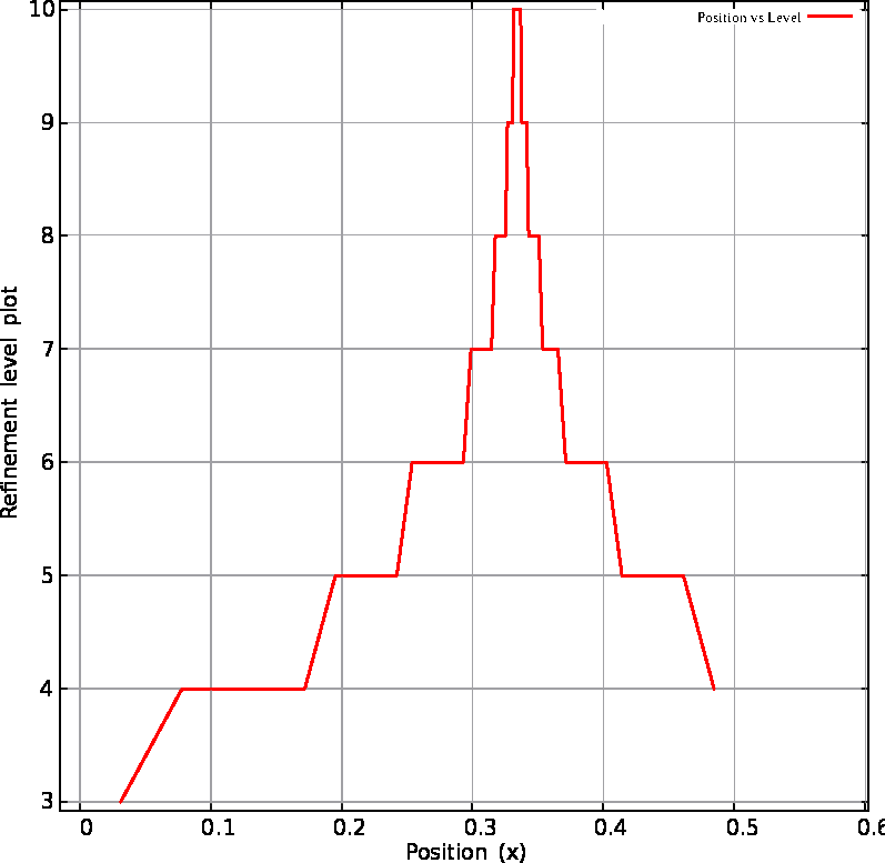 (a) Position vs Level |
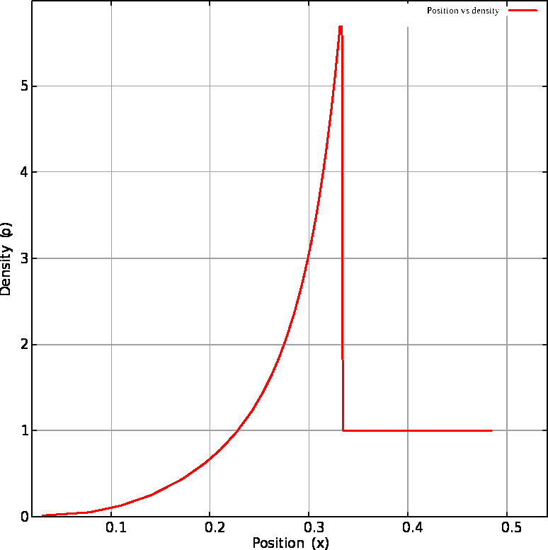 (b) Position vs Density |
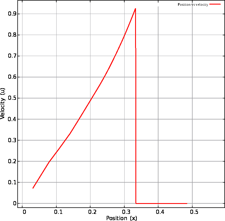 (c) Position vs Velocity |
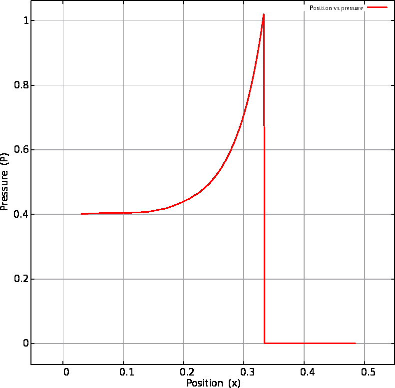 (d) Position vs Pressure |
Figure: Comparison of Sedov-Taylor 1D blast wave profiles for refinement levels, density, velocity, and pressure at different simulation parameters. The shock front is visible as a sharp jump in these physical quantities.
4 Compilation of 2D Sedov Simulation:
First you need to ’make clean the previously executed programs, in the ˜/ramses/bin and rerun the below command, whiling addressing the dimension value to be 2, and it will give you the executable file name ’ramses2d’.
You can now see ramses2d executable file inside bin directory.(mynewvenv) [golu@T430 bin]$ make clean rm -f *.o *.mod *.i (mynewvenv) [golu@T430 bin]$ ls clusters.mk Makefile ramses1d (mynewvenv) [golu@T430 bin]$ make NDIM=2Now lets have a look into our sedov2d input file, which is inside 'namelist/' directory. if you just do 'cat sedov2d.nml', you will be able to see what inside the file. Here we will try to edit this file. Right now if you see ''&OUTPUT_PARAMS'' its mentioned 'noutput=1', we change it to this value 'noutput=5' and and similarly for 'tout=1.0', which tell the boundary conditons at this time, we change this to 'tout=0.0625,0.125,0.25,0.5,1.0'. Which means, it will have different output for at several time. Now run the Ramses code for 2D, by executing 'ramses2d' file in ramses path and load the 'sedov2d.nml' .
You will get a ''Run completed'' in the output. Now again you get to notice you have gotton 6 outputs file because the first output file will auto make the initial condition at time=0.(mynewvenv) [golu@T430 ramses]$ bin/ramses2d namelist/sedov2d.nmlUsing this below command, you can check if you have gotten anything in the output file or not. If you see like some bigger numbers like 37k, 335K etc, means the position of the sedov2d blast wave has been obtained and you can check this outputs.
(mynewvenv) [golu@T430 ramses]$ ls -lh output_0000*/amr_*.out00001
-rw-r--r-- 1 golu golu  37K Feb  9 20:22 output_00001/amr_00001.out00001
-rw-r--r-- 1 golu golu 335K Feb  9 20:22 output_00002/amr_00002.out00001
-rw-r--r-- 1 golu golu 457K Feb  9 20:22 output_00003/amr_00003.out00001
-rw-r--r-- 1 golu golu 633K Feb  9 20:22 output_00004/amr_00004.out00001
-rw-r--r-- 1 golu golu 879K Feb  9 20:22 output_00005/amr_00005.out00001
-rw-r--r-- 1 golu golu 1.2M Feb  9 20:23 output_00006/amr_00006.out00001
4.1 Output Analysis for 2D:
For 2D, we have to need to have a python script so that we have check the outputs. For 1D it was simply a text file with data, which we had plotted. 1. First have a python script like this below,
(mynewvenv) [golu@T430 ramses]$ cat 3.py
import osyris
import matplotlib.pyplot as plt
 \# choose outputs you want
outputs = range(1, 7)   # 1, 2,3,4,5,6
for out in outputs:
    print(f"Processing output {out}...")
    data = osyris.RamsesDataset(out, path="./").load()
     plt.figure()  # new figure for each plot
     osyris.map(
        data["mesh"].layer("density"),
        norm="log",
        cmap="jet"
    )
    plt.savefig(f"out{out}-sedov2d.png")
    plt.close()   # free memory
Processing 1 files in ./output_00005
Loaded: 27262 cells, 0 particles.
Processing output 6...
Processing 1 files in ./output_00006
Loaded: 34198 cells, 0 particles.
- We had the value of output time 'tout=0.0625,0.125,0.25,0.5,1.0'. You can the outpust dictionary by, this means we have this all physical variable available in outputs, that we can model.
(mynewvenv) [golu@T430 output_00002]$ python Processing 1 files in ../output_00002 Loaded: 9874 cells, 0 particles. dict_keys(['level', 'cpu', 'dx', 'density', 'pressure', 'position', 'velocity', 'mass']) >>> - Python script for all at once. it will print “done” and save the output images.
import osyris
import numpy as np
import matplotlib.pyplot as plt
outputs = range(1,7)
for out in outputs:
print(f"Processing output {out}...")
data = osyris.RamsesDataset(out, path="./").load()
\# For level
plt.figure()
osyris.map(data["mesh"].layer("level"), cmap="viridis")
plt.savefig(f"out{out}-sedov2d-level.png")
plt.close()
\# For density
plt.figure()
osyris.map(data["mesh"].layer("density"), norm="log", cmap="jet")
plt.savefig(f"out{out}-density-new-jet.png")
plt.close()
\# For pressure
plt.figure()
osyris.map(data["mesh"].layer("pressure"), norm="log", cmap="jet")
plt.savefig(f"out{out}-sedov2d-pressure.png")
plt.close()
\# For mass
plt.figure()
osyris.map(data["mesh"].layer("mass"), norm="log", cmap="jet")
plt.savefig(f"out{out}-sedov2d-mass.png")
plt.close()
print("Done.")
Combine all images, output 4 from each variable, below command is to combine all four image and convert it to one image. further you can see the image generated. This image is like the one below, showing a comparison of position (x) against levels (lev), density (rho ), mass (m), and pressure (P). We will now plot for the velocity seperatly,as its have x and y axis parameter differently.
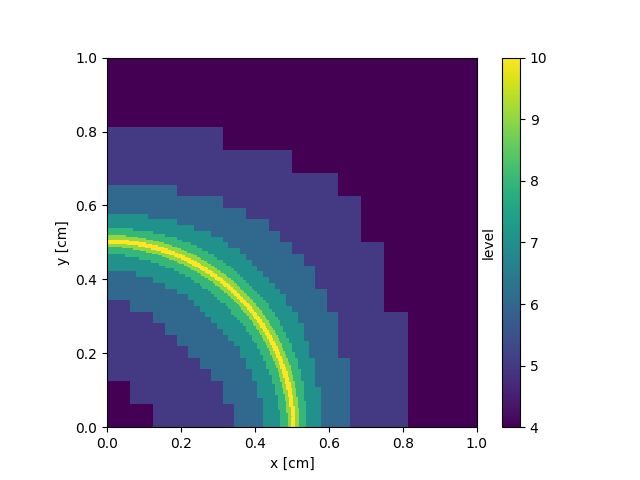
(a) Radius vs Level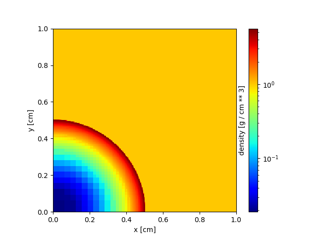
(b) Radius vs Density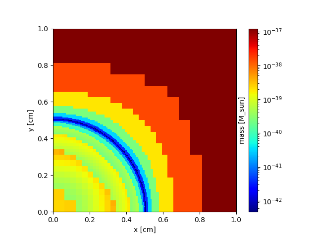
(c) Radius vs Mass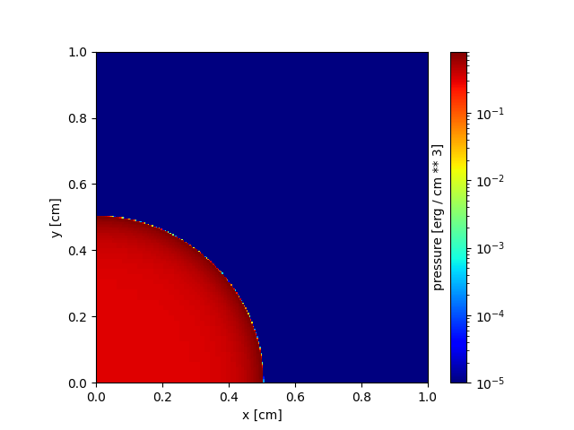
(d) Radius vs PressureFigure: Comparison of Sedov-Taylor 2D blast wave profiles for refinement levels, density, mass, and pressure against the radius (cm) of supernovea at different simulation parameters.
Now you can also have animation for this image, using this command for each. level gif [https://displ.nl/pb/sedov2d-level-40.gif||here], density gif [https://displ.nl/pb/sedov2d-density-40.gif||here], mass - git [https://displ.nl/pb/sedov2d-mass-40.gif||here] and pressure - gif [https://displ.nl/pb/sedov2d-pressure-40.gif||here]
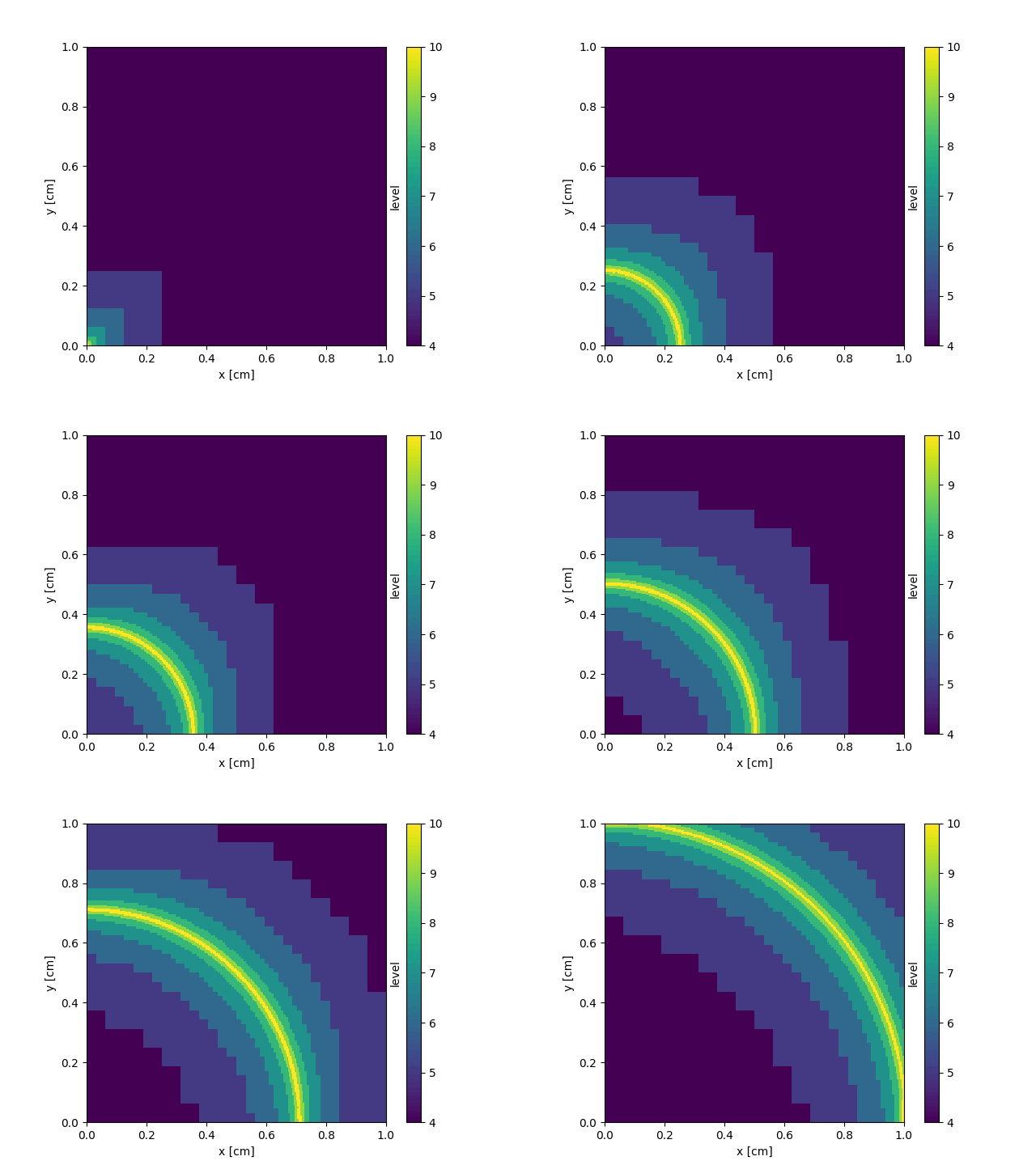 (a) Level Evolution |
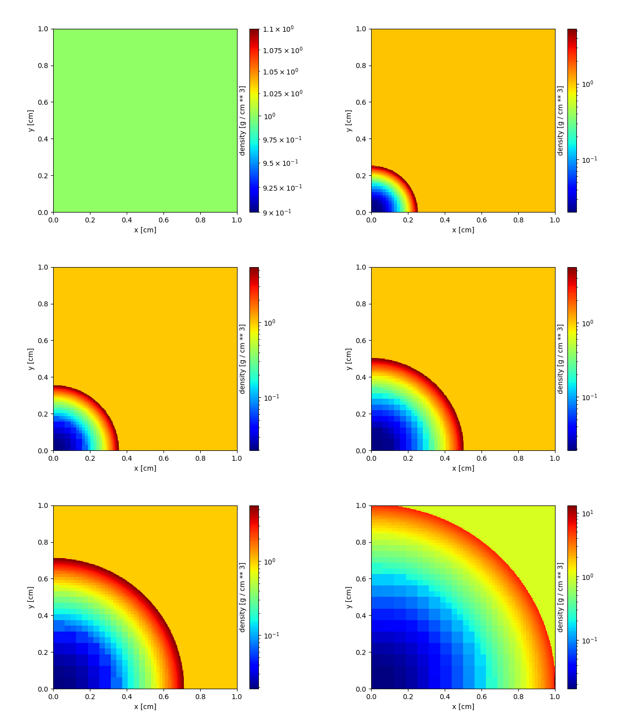 (b) Density Evolution |
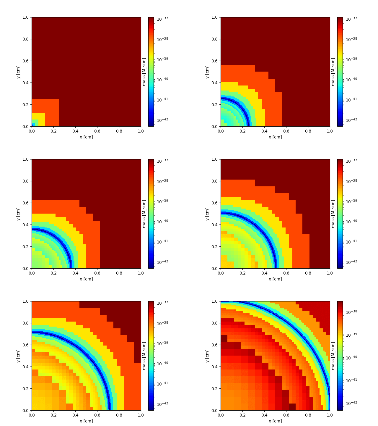 (c) Mass Evolution |
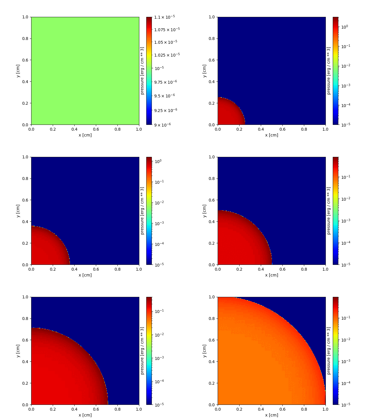 (d) Pressure Evolution |
Figure: Time evolution of 2D Sedov blast wave showing refinement level, density, mass distribution, and pressure.
4.2 Comparing 1D with 2D:
There are many things, we can carry out to analyze the output data. 1. Here one thing, we can compare using below script, this will help us understand both the spatial shock shape in 2D and how the density varies radially, allowing a direct comparison with the 1D solution.
(mynewvenv) [golu@T430 ramses]$ cat 1d-2d-comparision.py
import numpy as np
import matplotlib.pyplot as plt
import osyris
for nout in range(1, 7):
    print(f"Processing {nout}")
    data = osyris.RamsesDataset(nout, path="./").load()
    mesh = data["mesh"]
    fig = plt.figure(figsize=(12,4))
    ax1 = fig.add_subplot(121)
    ax2 = fig.add_subplot(122)
   \# ---- density (2D)
    osyris.map(
        mesh.layer("density"),
        norm="log",
        cmap="jet",
        ax=ax1
    )
    \# ---- radius vs density scatter (1D)
    r = mesh["position"].norm.values
    d = mesh["density"].values
    ax2.scatter(r, d, s=5)
    ax2.set_xlabel("radius")
    ax2.set_ylabel("density")
    fig.savefig(f"sedov_{nout:02d}.png", bbox_inches="tight")
    plt.close(fig)
we generate a figure that shows two types of visualizations for each timestep. On the left side shows the 2D density field, which illustrates the overall shock structure and symmetry. On the right side, the density is plotted as a function of radius, showing the radial shock for 1D profile.
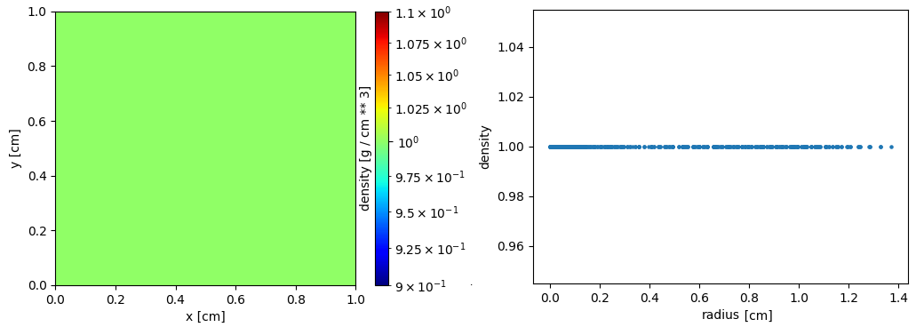
(a) 2D vs 1D at r = 0
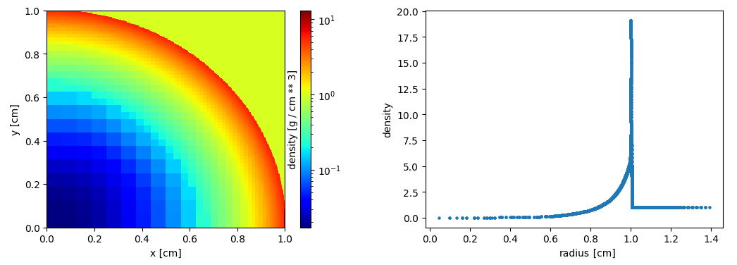
(b) 2D vs 1D at r = 1.0
Figure: Comparison of 2D Sedov-Taylor blast wave density profile against 1D plot showing density vs radius (cm) of supernova at different time. Figure (a) shows the initial radius r = 0, while Figure (b) represents the final stage at radius r = 1.
5 Executing 3D on HPC Cluster:
I am running inside HPC cluster now. I have used the same steps for executable file called 'ramses3d' and I compiled with 'sedov3d.nml' input file.
Once you compiled in your 3D input file. Its suggested to check whether the data outputs have been created or not using below command line. In my case, it says alot of data has been generated like 366M.
[c500@cometlogin(comet) ramses]$ ls -lh output_0000*/amr_*.out00001
-rw-r----- 1 c500 cometlogin 366M Feb 10 21:43 output_00001/amr_00001.out00001
-rw-r----- 1 c500 cometlogin 366M Feb 10 21:44 output_00002/amr_00002.out00001
-rw-r----- 1 c500 cometlogin 366M Feb 10 21:45 output_00003/amr_00003.out00001
-rw-r----- 1 c500 cometlogin 366M Feb 10 21:45 output_00004/amr_00004.out00001
-rw-r----- 1 c500 cometlogin 366M Feb 10 21:46 output_00005/amr_00005.out00001
-rw-r----- 1 c500 cometlogin 366M Feb 10 21:50 output_00006/amr_00006.out00001
Note for we cant use the 2D python script and do slicing manually. instead of that, for 3D RAMSES, yt is made exactly for this, hence we have install it by using “pip install yt” inside the virtual environment. our current tool Osyris is mainly designed for 2D maps (slice/projection).It does not provide real 3D rendering.