CamphorDynamics  Top-level Files of trunk

Intro

This is a directory of various interactive Pluto.jl notebooks that formed the basis for the study of,

1. Stationary and libration motion in two coupled rotors: Theoretical and experimental study - 10.1103/PhysRevE.110.064208.
2. Libration Motion In Coupled Rotors - Unpublished.

It also includes Makie snipets to interact and visualize the two camphor motion. This text follows the logical flow of explanining functions rather than the structure on the manuscript.

To clone this fossil repository and view locally, execute,

$ fossil clone https://fsl.displ.nl/camphor_dynamics 
$ cd camphor_dynamics
$ fossil ui

Setting Up Julia Environment

Most of the development has been done on julia 1.9.4 & 1.10, these can be installed using juliaup with the following,

$ juliaup add  1.9.4 
$ juliaup add  1.10 

One don't have to worry about the existing julia versions, because the particular environments can be activated exclusive to the Pluto.jl notebooks. There has been major change in Pluto.jl from 1.10 so I prefer starting Pluto in either of these versions,

$ julia +1.9.4   
$ julia> import Pluto; Pluto.run()

Dependency Checks

Below is the list of bare minimum dependencies to evolve the dynamical system,

# General environment
using PlutoUI, DelimitedFiles, LaTeXStrings, Plots;  gr(size=(400,400))
# For evolution
using DynamicalSystems, OrdinaryDiffEq, ProgressMeter, FFTW

Some of the scripts/notebooks have unique functions, in those cases additional dependencies are listed in the wiki below to make it executable.

Migration of Julia Environment

For the migration from one system to other, the following needs to be copied,

~/.julia/environment/v1.9/Manifest.toml
~/.julia/environment/v1.9/Project.toml
~/.julia/artifacts/v1.9
~/.julia/registries/v1.9
~/.julia/compiled/v1.9/

Although this will copy the compiled packages, most of the machines need to recompile again on the first run.

Structure of Notebooks

The notebooks are self contained with their problem definition and goal. Each of them have a section, "Parameters" that dynamically definies the system parameters.

Note: Julia enviornment path should be added manually instead of using Pluto's own environment, this is to use the system wide pre-compiled packages. Eg, the line needs to be modified according to the $USER,

Pkg.activate("/home/$USER/.julia/environments/v1.9/Project.toml")

rotor_param.jl

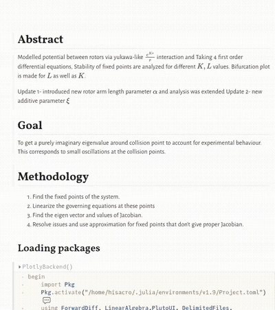
Fixed points of the system is catagorized in this notebook by finding the jacobian at these points. There is a simplification carried out to prevent jacobian vanishing at non-trivial points. This has been justified by comparing the approximation terms as well as an additive parameter. Demo below shows the overview of the notebook and explore the changes in eigenvalues at different configuration when system parameter is varied.

rotor_transcend_fixed.jl

Calculation of the fixed points of the system has been detailed along with two different cases. For the initial study, only one of the conditions is taken into account.

rotor_expo.jl

Documentation for choosing the valid initial conditions based on two methodologies. Both of these methods incorporte dynamic point & click function within a plot in Pluto notebook.

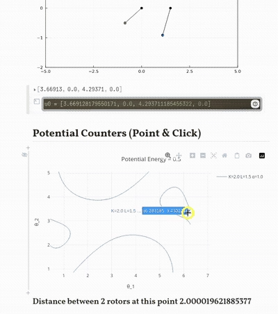
One of them slices the potential countour at the choosen energy and allows to choose the set of $(theta_1, theta_2)$ that lies on it. With the possibility of fixing p2 (omega_2) by the user, the function outputs the set of initial conditions satisfying the fixed energy. It also shows the starting configuration of rotors and evolves the system to calculte largest lyaponov cofficient.

rotor_energy_init.jl

Dynamical system is numerically integrated using the appropriate algorithm (Verner's) with the time step of $10^-4$. Multi axis time series plots is constructed after evolution.

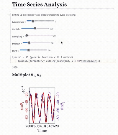
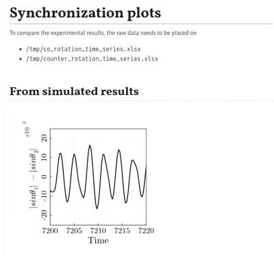
Synchronization parameter is plotted against time. Relative phases of angles are plotted as sinusoidal functions to correlate with the synchronization.

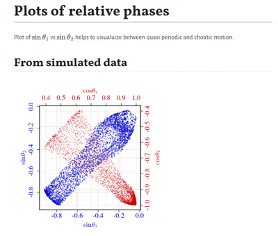
Three miscellaneous fucntions are also included, one calculates the largest Lyapuno Exponent for the choosen initial condition. The second function converts evolution from time to frequency space using Fast Fourier Transforms. Final function help to visualize the rotor system by manually adjusting the time step with Pluto's NumberField but this was left out intentionally after first revision due to redunany with GLMakie's standalone function.

The figures in the article are generated using functions from this notebook.

rotor_lya.jl

Fixing the energy of the system, all the valid initial conditions are calculated. It uses IntervalRootFinding algorithm to search through the domain space. It's an analog of Point & Click function in rotor_expo.jl. Following demo shows dynamics adjustment of bounding regions of phase trajectories.

When a phase space trajectory is constructed, the enclosing countours shows the validity of the plot. By evolving distance between the two rotors and the potential energy as the function of time, libration types are distinguished.

bif_area.jl

The closed contours at different energy levels in the phase space can be associated with the two libration types seen in the system. Plotting area of these contour vs energy can be helpful to associate the birth of these libration types and changes in the dynamics associated to them. Demo below explores the changes in area of contour plot when system parameter, L - pivot length is increased from 1.4 to 1.6.

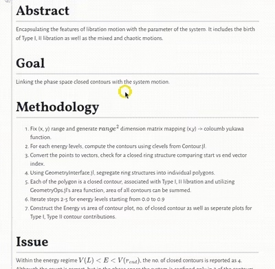
This notebook relies on Contour.jl, GeoInterface.jl and GemetryOps.jl.

bif_energy.jl

System characteristics are grouped in different energy regimes. The function to find r_end, r corresponding to the maxima of the potential is outlined. The methodology and calcuation of r_ex, extrema of distance between rotors at an energy level is documented. Demo below shows the variation in the plot of r_ex as a function of energy, when system parameters L and K are varied.

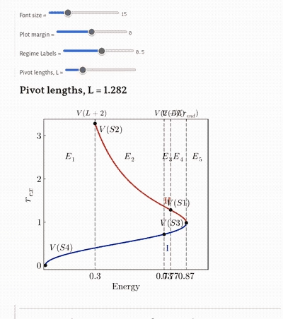
TODO

[ ] Complete Checklist
	[x] rotor_param.jl 
	[x] rotor_transcend_fixed.jl 
	[x] rotor_expo.jl 
	[x] rotor_energy_init.jl 
	[x] rotor_lya.jl 
	[x] bif_area.jl 
	[x] rotor_rvalue_backup.jl (same as rotor_lya.jl)
	[x] libr_bif.jl (should be in bif_area.jl)
	[x] lya_data (raw data of initial conditions with a<=0.5)
	[x] heatmap.jl (sample notebook)
	[x] bifn.jl (not a notebook)
	[x] rotor_hamil_order3_simple.ji 
	[x] sync_order3_today.ji 
	[x] sync_order3_subfig_theta_series.ji 
	[x] bif_energy.jl
	[ ] bifn_energy_single.jl
   	[ ] rotor_transcend_fixed.jl -  Libration
	[x] points_d.jl
	[x] sync_order3_bkup.ji
[X] Organize wiki pages
[X] Add notebook demos 
[X] Add makie demos
[ ] radian ticks in GLMakie
[ ] bif_energy.jl migration
	[ ] Compilation of IntervalRootFinding.jl in v1.9
	[ ] Rewrite rmax() function for v1.10+