
This repository is collection of julia notebooks (Pluto.jl) and simulation scripts (Makie.jl) to study rotor dynamics. It is also the code basis for the master dissertation - Understanding Two Coupled Rotors, the article - Stationary and libration motion in two coupled rotors and an unfinished manuscript - Libration Motion In Coupled Rotors. Interacting camphor strips were modeled as rotors in these studies, hence the title.
The Need?
The theory behind the system I studied has been documented, but the code base was not. When I begun the study, Julia as a language was new to me and due to strict time constrain of my masters, the main objective was to make it work rather than make it clean and readable. Even so, most of the days has been spent reading documentations and going through Julia forum interactions. Infact, functions written here were brainchild of interactions from the Julia package developers themselves. Unfortunately, some of them were not documented or not landed in the package upstream. To name a few,
- Point & Click function inside Pluto.jl notebook. (uses PlutoPlotly.jl) - rotor_expo.jl
- Calculating Area of the potential contours. (uses Contour.jl, GeometryOps.jl & GeoInterface.jl) - bif_area.jl
I wanted communal efforts not to vanish into oblivion, hence the intent of this repository.
Resources
A heavy influence comes from JuliaDynamics. System evolution and parameters are set with DynamicalSystems.jl, this becomes the initialization statement in all the notebooks and scripts. Makie interactive scripts were modified and built on top of Datseris/makie_tutorial.jl.
This study and development wouldn't have been possible without the guidance of my supervisors, Prof. Awadhesh Prasad and Prof. Sangeeta D. Gadre. I'm also grateful for the feedback from my collaborators and Julia community for helping me optimize the scripts.
Rest of the wiki pages document the functions used to uncover the intricacies of the studied system (Modified Coulomb-Yukawa Potential). Nevertheless, almost all the functions can be adopted for any other rotor systems by replacing the interacting potential.
Modified Coulomb-Yukawa Potential
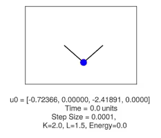
The initial problem statement was on studying the rotor system at the collision points. The details on coming up with the interaction potential has been documented in the article. With this form of potential, the system undergoes small oscillations at collision points as follows,
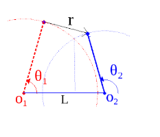
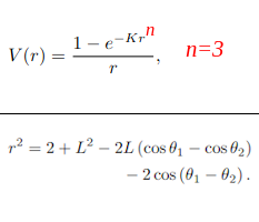
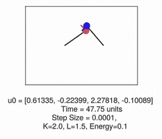
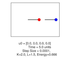
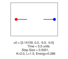
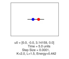
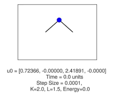
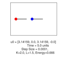
To proceed further with the study, all the fixed point of this system were identified notebook - rotor_transcend_fixed.jl. Since the system is conservative, the points are classified either as saddle or center. Following are the system configurations, (mirrored initial condition are grouped together)
| S1 | S2 | S3 | S4 |
|---|---|---|---|
 |
 |
 |
 |
 |
 |
||
| saddle | center | saddle | center |
In order to classify the fixed points, eigenvalues of Jacobian at these configurations are calculated in the notebook - rotor_param.jl. For the configuration S4, the potential is Taylor expanded before calculating Jacobian to avoid singularities. The dynamics plots for eigenvalues of Jacobian at these configurations are also present on the notebook.
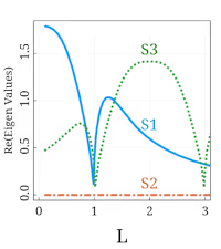
The validity of evolution has been verfied in rotor_energy_init.jl. This notebook also includes functions to plot the time series of rotors, relative phases as well as verification of synchronization condition.
Potential Contours
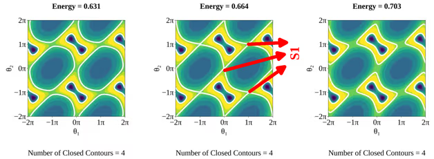
The second part of the study tried to answer the bounded oscillations seen in the system. It starts off with the closer look of potential contours in the phase space. What follows below is the sequence of contour cross sections at each energy levels,
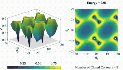
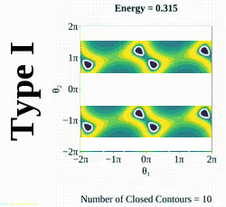
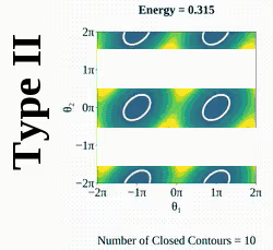
Within the same energy level, there are two types of closed contours (since the axis is in radians, mirror contours are grouped together). The one that emerges first is named as "Type I" and the second one as "Type II"
Libration Types
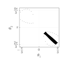
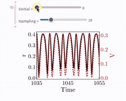
To figure the distinct characteristics in Type I and II, the initial condition are chosen within these contours and made to evolve. The plot of phase space trajectories and evolution of distance between rotors vs potential energy is tabulated below for system energy - 0.315,
| Type I | Type II | |
|---|---|---|
  |
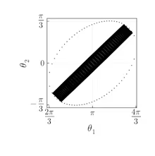 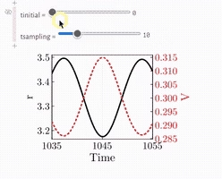 |
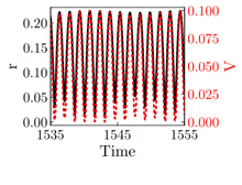
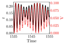
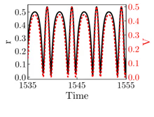
In the Type I oscillations, maxima of distance between the rotors and potential energy coincides throughout the evolution while in Type II extrema negates each other.
Type I
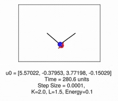
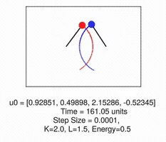
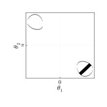
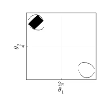
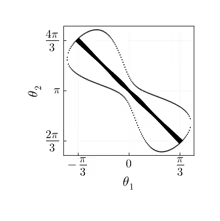
Within Type I, there are small as well as large oscillations. Small oscillation corresponds to the evolution inside either of the Type I mirrored contours. Large oscillation occur when these two contours are merged into one and system is confined inside.
| Type I (small) | Type I (small) | Type I (large) | |
|---|---|---|---|
| Simulations | |
 |
 |
| Phase space trajectory |
 |
 |
 |
| Evolution plot of r vs V |
 |
 |
 |
Type I large oscillations start to appear in the system only after a certain energy, this is evident in the potential contour sequences.
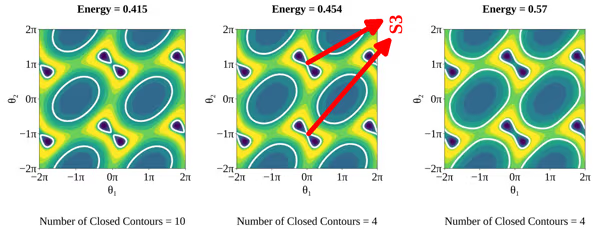
The point at which the Type I closed contours merged is identified as S3. The distance of rotors ends at this configuration is 2-L, where L is distance between pivots. This helps to figure the transition energy level in Type I as V(2-L), since potential is a function of r.
Type II
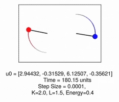
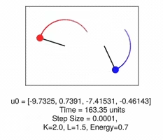
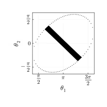
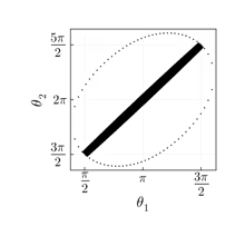
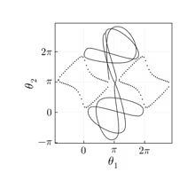
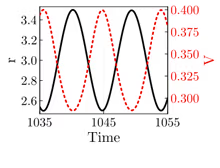
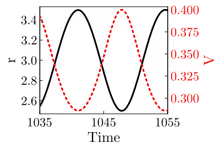
Similarly in Type II, there are simple and mixed motions, In simple Type II motion, both the rotors are confined by a certain angle preventing them to make a 2pi oscillations. In the mixed motion, either one of the rotors crosses the 2pi mark, making a full oscillation.
| Type II | Type II | Type II (mixed) | |
|---|---|---|---|
| Simulations | 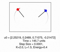 |
 |
 |
| Phase space trajectory |
 |
 |
 |
| Evolution plot of r vs V |
 |
 |
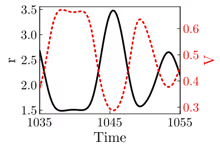 |
Type II mixed oscillations start to appear after merging of contours at S1. The distance of rotors ends at this configuration is L, hence the energy level is V(L). Following contour sequences depict the same.
Unbounded & uncoupled Motion.
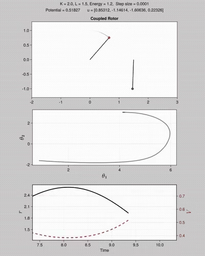
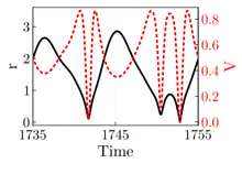
Beyond the energy level, the system has no bounded motion (constrain on angle) due to absence of closed contours. This can be seen on the Makie simulations, following shows 2 additional subplots for phase space and r vs V evolution.
 |
 |
|---|
The trends of r vs V evolutionary plots seen in Type I, II oscillation gets disrupted. As a consequence, maxima of r and V doesn't coincide throughout the evolution but interchanges after a period of time. This leads to uncoupled motion, relative phase plots make this more evident.
The energy when these motion occur has been identified as V(r_end) and the calculation or r_end can be found in the notebook - bif_energy.jl (static page).
Combined Results
To quantify the difference between the libration types, area of the closed contours associated with each of the types is considered as a parameter. The following subplots show how area and no. of. closed contours vary as a function of system energy.
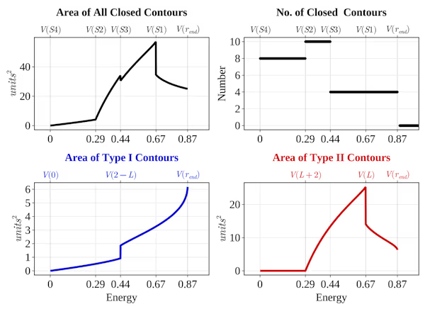
Methodology and calculation are present in the notebook bif_area.jl. There is also a demo present in the wiki, showcasing how the pivot length - L, changes the characteristics of these contour area plots.
Contour Area Consequence
In the contour area plots, there are steep inclines present at certain energy levels. These occurs at the levels when contours merge, in the Type I subplot this corresponds to the levels after emergence of V(S3) while in Type II, energy levels after V(S1) configuration. The top axis lists the potential as a function of r, distance between the rotors. Hence, V(S3) and V(S1) are analogous to V(2-L) and V(L) respectively. This is possible since V, potential can be written as fucntion of theta_1, theta_2 (former) or function of r (later).
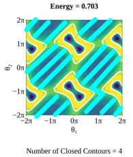
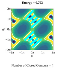
Due to the way the closed closed are calculated, an abnormality rises in Type II contours area calculation. Details have been explained in the notebook - bif_area.jl, for the completeness it's reiterated below,

This is the reason for the dip in Type II subplot at V(S1). Following energy contours plot details the associated issue, (the crossed cyan lines denote Type II contours)
| Confined phase space of Type II libration motion |
Confined phase space that script considers for Type II closed contour area calculation |
|
|---|---|---|
 |
 |
Although area parameter satisfies the motive of capturing the transition energy level and associated configuration, it complicates the problem. There are workarounds to report the phase space confinement area rather than area of closed contours. However, a new system parameter, r_ex is preferred over this approach.
Energy Regimes
r_ex is the maxima of distance between the rotors at the particular energy level. The methodology and calculations has been documented in the notebook - bif_energy.jl. The results from studying the energy contours and system evolution are summarized in the table below (adopted from manuscript), characteristics of the system are grouped together in different energy regimes.
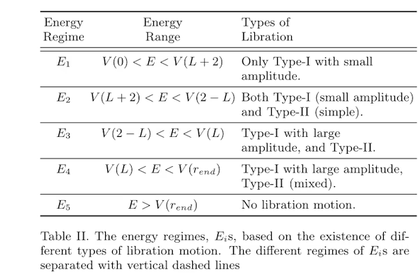
The following plot, r_ex as the function of energy summarizes this study. The bottom x-axis of the plot corresponds to energy of the system with the parameters, K=2.0 and L=1.5. The top x-axis are analytical expressions to calculate the energy, since potential energy is function of "r", each of the values (0, 2-L, L+2, L, r_end) denote distance between rotor ends.
The labels S1 to S4 corresponds to the configurations reported in the first part of study. Since these are function of $theta_1, theta_2$, the value of r is calculated for these configuration and then the corresponding energy, V. It's found from the contour plots as well as from the calculation of r_ex, S4 and S3 are associated with Type I libration, whereas S2 and S1 lies on the Type II libration solution curve.
Type I and Type II oscillation merge at V(r_end), beyond this energy level libration motion is not present in the system.
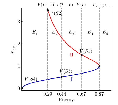
There is also an interactive demo of the notebook - bif_energy.jl showcasing the changes in $r_ex$ plot when system parameter, L, pivot length is varied.